Computational Graphs & Backward Propagation

Date : 2022.10.09

 

*The contents of this book is heavily based on Stanford University’s CS231n course.

 

[Improving Efficiency]

So far, we've used multivariable calculus techniques such as differentiation and gradients to derive the “slope of the loss function for weights.”

 

Implementing a new method called “Backward Propagation of Errors (backpropagation)” will increase efficiency in the SGD process.

 

[Computational Graphs]

A computational graph represents mathematical processes in the form of graphs. Rather than complex equations, we will use graphs to represent both forward & backward propagation.

 

Why use Computational Graphs?

 

The upside of graphs is the structure itself. Graphs are composed of nodes and edges. In computational graphs, the forward propagation is from left to right and each node’s calculation is affected only by directly connected nodes. By connecting the nodes we can calculate how one node affects another in long distances. Overall, graphs allow us to break down the entire process into node units.

 

[Forward & Backward Propagation of Computational Graphs]

 

We can easily calculate how one node’s value changes another node’s value which is pretty much the definition of differentiation.

 

[Forward & Backward Propagation in Depth]

Backward propagation follows the chain rule.

 

[Backward Propagation]

 

[Backward Propagation as Differentiation]

 

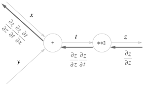
The node carries a mathematical calculation and the edge carries the value. Thus, there are different backward propagations for different types of nodes.

 

1. Addition Node :

 

[Backward Propagation for Addition]

 

[Example]

 

The backward propagation for addition nodes is the same as the forward propagation input.

 

[Addition Node Code]

 

1. Multiplication Node :

 

[Multiplication Node Differentiation]

 

[Backward Propagation for Multiplication]

 

The backward propagation for multiplication nodes require a swapped value multiplication of the forward inputs. Since the backward inputs rely on the forward inputs, we will save the forward inputs for the backward function.

 

[Multiplication Node Code]

 

[Propagations of Addition & Multiplication]

 

[Apple & Orange Example Code]

 

1. ReLU :

While the addition and multiplication propagations are basic calculations, by combining several nodes we can also build more complex graphs for nodes.

 

[ReLu Graph]

 

[ReLU Node Code]

*Line 42 : If x is true (<= 0), line 44 converts the true values into 0.

 

The mask instance saves the trouble of implementing an if-statement for converting variables less than 0 into 0. Since ReLU only has outputs of either 0 or 1 we use the mask function to separate the 0’s and 1’s.

 

1. Sigmoid :

 

[Sigmoid Propagation]

 

[Sigmoid Propagation]

 

[Sigmoid Node Code]

 

1. Affine :

Before implementing the Affine layer, let’s quickly review the network structure.

 

[Network w/ Affine, ReLU, and Softmax]

 

Each function we program corresponds to a layer of the entire. As given in the CNN above the Affine transformation (or layer) is built by np.dot().

 

[Affine Layer Graph]

 

Affine transformation is tricky. The components are matrices. Understanding the differences between ‘dot’ node and ‘multiplication’ node is crucial. Since, matrix calculation no longer consists the ‘scalar’ properties new rules apply for backward (differentiation).

 

[Affine Layer Backward Propagation]

 

[Affine Node Differentiation]

 

[Affine Node Code]

 

1. Softmax-with-Loss :

The softmax function lies in the last layer. It’s the final step of the CNN in which the network outputs a normalized probability for each case.

 

Since our output cases are numbers (0~9), both the number of input and output variables of the softmax function is 10.

 

*Note: The CNN undergoes two different stages.

The first one is the learning stage in which we feed a considerable amount of data to the CNN and find the optimal weights and hyperparameters. This stage requires softmax function’s normalization because we compare the normalized outputs with the one-hot encoded answer labels.
The second one is the testing (prediction) stage in which we test data with the optimized CNN. This stage does not require the softmax function since we only need the outputs from the last Affine layer. The maximum output from this layer is the final result.

 

[Softmax-with-Loss Layer]

 

[Softmax-with-Loss Graph]

 

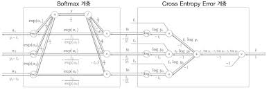
We combined the softmax and loss function (CEE) because our original method for finding gradients relies on the loss function as well.

 

The key point is the output of the backward propagation. We get a simple mathematical equation for backward propagation. This is remarkable. The entire purpose of using computational graphs and conducting backward propagation was to INCREASE EFFICIENCY in optimizing weights. With the established backward propagation we no longer need to differentiate every weight for gradients.

 

[Softmax-with-Loss Node Code]

Now that we’ve completed building the lego blocks for our building, in the following post we’re going to put together the blocks.