Date : 2022.09.23
*The contents of this book is heavily based on Stanford University’s CS231n course.
[Data Modeling]
The data modeling process can be separated into 2 major steps: Learning and Testing.
In the learning process our goal is to establish a neural network with high precision. We can control a few variables that will affect the model. The first control variable is the Weight Variable, and weight optimization requires the use of learning data. There are several ways of optimization and our main method is Stochastic Gradient Descent (SGD) which uses gradients (functions).
[Data]
MNIST is a set of images. Images have certain features that establish a pattern for our model. An image's feature can be written in vectors which is the key ingredient for categorical algorithms such as SVM and KNN (not deep learning). In these cases, it is our job to convert images to vectors using the ‘features’ as our guidelines. However, deep learning categorizes images based on what it learns from studying thousands of data.
Let’s dive into end-to-end machine learning.
As mentioned above, we first want to separate our data into 2 sets.
- Training Data
- Test Data
[Loss Function]
As mentioned, we feed the weights into the model to reach optimized values. The question is “What weights are the best?” “How do we define ‘best’?”
We’re going to use the loss function. There are 2 components of the loss function.
First is the Sum of Squares of Error, SEE.


The second component is Cross Entropy Error, CEE.

t is the answer in the form of one-hot encoding and y is the outcome of the neural network's softmax layer.

According to the graph above, as the outcome value x decreases the CEE value increases. Conversely, as the outcome value is higher (= higher probability) the CEE decreases which means the outcome is closer to the correct answer. In conclusion, the CEE is smaller if our outcome probability is higher.

We should remind ourselves that the ultimate goal of this project is to develop a high precision image categorization network. One of the key components affecting the precision are the weights. The weights represents the importance of a characteristic when analyzing an image.
Typically each characteristic has different weights. The characteristics are represented as nodes in our neural network. Thus, we work with multiple weights and multiple loss functions for each variable. We want to minimize the loss (incorrectness) of each loss function and the optimal way is relying on gradients of the loss functions.
[Gradient Descent Method]
The gradients suggests a direction for the CNN to modify the weights.

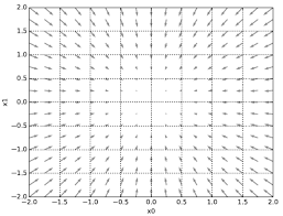
The vector field points to the center, which is the point that decreases the function output the most. In other words the gradients point in the direction that is closest to finding the minimum value. This hints at why we differentiate the loss function rather than directly use the xy values. In an actual neural network there are multiple weight variables and loss functions that go along with it. Thus it is inefficient to pinpoint the minimum value by randomly exploring the slopes. A more efficient method of using gradients is called the gradient descent method.

𝜂 (eta) is the learning rate, which is a hyperparameter we will later explore. The rest of the equation is quite intuitive.

Learning rate is a hyperparameter. Hyperparameters are set by the programmer. These differ from variables such as weight and bias. To find the best hyperparameter we should test multiple candidates and compare their precision. Later we will also study how to set optimal hyperparameters for better efficiency and precision.


The gradients per weight is the relation between the weights and final output. For example, the 0.15 in W[0][1] position means that h change in W[0][1] changes the final outcome by 0.15h.
'Tech Development > Deep Learning (CNN)' 카테고리의 다른 글
| Computational Graphs & Backward Propagation (0) | 2022.10.24 |
|---|---|
| SGD, Epochs, and Accuracy Testing (0) | 2022.10.22 |
| Activation Functions (Sigmoid, ReLU, Step) & Neural Networks (0) | 2022.10.14 |
| Perceptrons, Equations, and Gates (0) | 2022.10.08 |
| Getting Familiar with Numpy & Matplotlib (0) | 2022.10.08 |


댓글